So far we have seen two concentration bounds for scalar random variables: Markov and Chernoff. For our sort of applications, these are by far the most useful. In most introductory probability courses, you are likely to see another inequality, which is Chebyshev’s inequality. Its strength lies between the Markov and Chernoff inequalities: the concentration bounds we get from Chebyshev is usually better than Markov but worse than Chernoff. On the other hand, Chebyshev requires stronger hypotheses than Markov but weaker hypotheses than Chernoff.
1. Variance
We begin by reviewing variance, and other related notions, which should be familiar from an introductory probability course. The variance of a random variable  is
is
![\displaystyle \begin{array}{rcl} {\mathrm{Var}}[X] ~=~ {\mathrm E}\Big[ \big(X-{\mathrm E}[X]\big)^2 \Big] ~=~ {\mathrm E}[ X^2 ] - {\mathrm E}[X]^2. \end{array}](https://s0.wp.com/latex.php?latex=%5Cdisplaystyle+%5Cbegin%7Barray%7D%7Brcl%7D+%7B%5Cmathrm%7BVar%7D%7D%5BX%5D+%7E%3D%7E+%7B%5Cmathrm+E%7D%5CBig%5B+%5Cbig%28X-%7B%5Cmathrm+E%7D%5BX%5D%5Cbig%29%5E2+%5CBig%5D+%7E%3D%7E+%7B%5Cmathrm+E%7D%5B+X%5E2+%5D+-+%7B%5Cmathrm+E%7D%5BX%5D%5E2.+%5Cend%7Barray%7D+&bg=ffffff&fg=000000&s=0&c=20201002)
The covariance between two random variables and  is
is
![\displaystyle {\mathrm{Cov}}[X,Y] ~=~ {\mathrm E}\Big[ \big(X-{\mathrm E}[X]\big) \big(Y-{\mathrm E}[Y]\big) \Big] ~=~ {\mathrm E}[XY] - {\mathrm E}[X]{\mathrm E}[Y].](https://s0.wp.com/latex.php?latex=%5Cdisplaystyle+%7B%5Cmathrm%7BCov%7D%7D%5BX%2CY%5D+%7E%3D%7E+%7B%5Cmathrm+E%7D%5CBig%5B+%5Cbig%28X-%7B%5Cmathrm+E%7D%5BX%5D%5Cbig%29+%5Cbig%28Y-%7B%5Cmathrm+E%7D%5BY%5D%5Cbig%29+%5CBig%5D+%7E%3D%7E+%7B%5Cmathrm+E%7D%5BXY%5D+-+%7B%5Cmathrm+E%7D%5BX%5D%7B%5Cmathrm+E%7D%5BY%5D.+&bg=ffffff&fg=000000&s=0&c=20201002)
This gives some measure of the correlation between and .
Here are some properties of variance and covariance that follow from the definitions by simple calculations.
Claim 1 If and are independent then ![{{\mathrm{Cov}}[X,Y] = 0}](https://s0.wp.com/latex.php?latex=%7B%7B%5Cmathrm%7BCov%7D%7D%5BX%2CY%5D+%3D+0%7D&bg=ffffff&fg=000000&s=0&c=20201002) .
.
Claim 2 ![{{\mathrm{Cov}}[X+Y,Z] = {\mathrm{Cov}}[X,Z] + {\mathrm{Cov}}[Y,Z]}](https://s0.wp.com/latex.php?latex=%7B%7B%5Cmathrm%7BCov%7D%7D%5BX%2BY%2CZ%5D+%3D+%7B%5Cmathrm%7BCov%7D%7D%5BX%2CZ%5D+%2B+%7B%5Cmathrm%7BCov%7D%7D%5BY%2CZ%5D%7D&bg=ffffff&fg=000000&s=0&c=20201002) .
.
More generally, induction shows
Claim 3 ![{{\mathrm{Cov}}[\sum_i X_i,Z] = \sum_i {\mathrm{Cov}}[X_i,Z]}](https://s0.wp.com/latex.php?latex=%7B%7B%5Cmathrm%7BCov%7D%7D%5B%5Csum_i+X_i%2CZ%5D+%3D+%5Csum_i+%7B%5Cmathrm%7BCov%7D%7D%5BX_i%2CZ%5D%7D&bg=ffffff&fg=000000&s=0&c=20201002) .
.
Claim 4 ![{{\mathrm{Var}}[X+Y] = {\mathrm{Var}}[X] + {\mathrm{Var}}[Y] + 2 \cdot {\mathrm{Cov}}[X,Y]}](https://s0.wp.com/latex.php?latex=%7B%7B%5Cmathrm%7BVar%7D%7D%5BX%2BY%5D+%3D+%7B%5Cmathrm%7BVar%7D%7D%5BX%5D+%2B+%7B%5Cmathrm%7BVar%7D%7D%5BY%5D+%2B+2+%5Ccdot+%7B%5Cmathrm%7BCov%7D%7D%5BX%2CY%5D%7D&bg=ffffff&fg=000000&s=0&c=20201002) .
.
More generally, induction shows
Claim 5 Let  be arbitrary random variables. Then
![\displaystyle {\mathrm{Var}}\Bigg[\sum_{i=1}^n X_i\Bigg] ~=~ \sum_{i=1}^n {\mathrm{Var}}[X_i] + 2 \sum_{i=1}^n \sum_{j>i} {\mathrm{Cov}}[X_i,X_j].](https://s0.wp.com/latex.php?latex=%5Cdisplaystyle+%7B%5Cmathrm%7BVar%7D%7D%5CBigg%5B%5Csum_%7Bi%3D1%7D%5En+X_i%5CBigg%5D+%7E%3D%7E+%5Csum_%7Bi%3D1%7D%5En+%7B%5Cmathrm%7BVar%7D%7D%5BX_i%5D+%2B+2+%5Csum_%7Bi%3D1%7D%5En+%5Csum_%7Bj%3Ei%7D+%7B%5Cmathrm%7BCov%7D%7D%5BX_i%2CX_j%5D.+&bg=ffffff&fg=000000&s=0&c=20201002)
In particular,
Claim 6 Let be mutually independent random variables. Then ![{ {\mathrm{Var}}[\sum_{i=1}^n X_i]~= \sum_{i=1}^n {\mathrm{Var}}[X_i] }](https://s0.wp.com/latex.php?latex=%7B+%7B%5Cmathrm%7BVar%7D%7D%5B%5Csum_%7Bi%3D1%7D%5En+X_i%5D%7E%3D+%5Csum_%7Bi%3D1%7D%5En+%7B%5Cmathrm%7BVar%7D%7D%5BX_i%5D+%7D&bg=ffffff&fg=000000&s=0&c=20201002) .
.
2. Chebyshev’s Inequality
Chebyshev’s inequality you’ve also presumably seen before. It is a 1-line consequence of Markov’s inequality.
Theorem 7 For any  ,
,
![\displaystyle {\mathrm{Pr}}\Big[ \big|X-{\mathrm E}[X]\big|\geq t \Big] ~\leq~ \frac{{\mathrm{Var}}[X]}{t^2}.](https://s0.wp.com/latex.php?latex=%5Cdisplaystyle+%7B%5Cmathrm%7BPr%7D%7D%5CBig%5B+%5Cbig%7CX-%7B%5Cmathrm+E%7D%5BX%5D%5Cbig%7C%5Cgeq+t+%5CBig%5D+%7E%5Cleq%7E+%5Cfrac%7B%7B%5Cmathrm%7BVar%7D%7D%5BX%5D%7D%7Bt%5E2%7D.+&bg=ffffff&fg=000000&s=0&c=20201002)
Proof:
![\displaystyle {\mathrm{Pr}}\Big[ \big|X-{\mathrm E}[X]\big|\geq t \Big] ~=~ {\mathrm{Pr}}\Big[ \big(X-{\mathrm E}[X]\big)^2\geq t^2 \Big] ~\leq~ \frac{ {\mathrm E}[ \big(X-{\mathrm E}[X]\big)^2 ]}{t^2} ~=~ \frac{ {\mathrm{Var}}[ X ]}{t^2},](https://s0.wp.com/latex.php?latex=%5Cdisplaystyle+%7B%5Cmathrm%7BPr%7D%7D%5CBig%5B+%5Cbig%7CX-%7B%5Cmathrm+E%7D%5BX%5D%5Cbig%7C%5Cgeq+t+%5CBig%5D+%7E%3D%7E+%7B%5Cmathrm%7BPr%7D%7D%5CBig%5B+%5Cbig%28X-%7B%5Cmathrm+E%7D%5BX%5D%5Cbig%29%5E2%5Cgeq+t%5E2+%5CBig%5D+%7E%5Cleq%7E+%5Cfrac%7B+%7B%5Cmathrm+E%7D%5B+%5Cbig%28X-%7B%5Cmathrm+E%7D%5BX%5D%5Cbig%29%5E2+%5D%7D%7Bt%5E2%7D+%7E%3D%7E+%5Cfrac%7B+%7B%5Cmathrm%7BVar%7D%7D%5B+X+%5D%7D%7Bt%5E2%7D%2C+&bg=ffffff&fg=000000&s=0&c=20201002)
where the inequality is by Markov’s inequality. 
As a quick example, suppose we independently flip  fair coins. What’s the probability that we see at least
  heads? Let
  be the indictator random variable of the event “
 th toss is heads”. Let
 ![{\mu = {\mathrm E}[\sum_i X_i] = n/2}](https://s0.wp.com/latex.php?latex=%7B%5Cmu+%3D+%7B%5Cmathrm+E%7D%5B%5Csum_i+X_i%5D+%3D+n%2F2%7D&bg=ffffff&fg=000000&s=0&c=20201002) . So we want to analyze
. So we want to analyze ![{{\mathrm{Pr}}[ \sum_i X_i - \mu \geq n/4 ]}](https://s0.wp.com/latex.php?latex=%7B%7B%5Cmathrm%7BPr%7D%7D%5B+%5Csum_i+X_i+-+%5Cmu+%5Cgeq+n%2F4+%5D%7D&bg=ffffff&fg=000000&s=0&c=20201002) .
.
Bound from Chebyshev: Note that
![\displaystyle {\mathrm{Var}}[X_i] ~=~ {\mathrm E}[X_i^2] - {\mathrm E}[X_i]^2 ~=~ 1/2 - 1/4 ~=~ 1/4.](https://s0.wp.com/latex.php?latex=%5Cdisplaystyle+%7B%5Cmathrm%7BVar%7D%7D%5BX_i%5D+%7E%3D%7E+%7B%5Cmathrm+E%7D%5BX_i%5E2%5D+-+%7B%5Cmathrm+E%7D%5BX_i%5D%5E2+%7E%3D%7E+1%2F2+-+1%2F4+%7E%3D%7E+1%2F4.+&bg=ffffff&fg=000000&s=0&c=20201002)
By independence,
![\displaystyle {\mathrm{Var}}[{\textstyle \sum_i X_i}] ~=~ \sum_i {\mathrm{Var}}[X_i] ~=~ n/4.](https://s0.wp.com/latex.php?latex=%5Cdisplaystyle+%7B%5Cmathrm%7BVar%7D%7D%5B%7B%5Ctextstyle+%5Csum_i+X_i%7D%5D+%7E%3D%7E+%5Csum_i+%7B%5Cmathrm%7BVar%7D%7D%5BX_i%5D+%7E%3D%7E+n%2F4.+&bg=ffffff&fg=000000&s=0&c=20201002)
By Chebyshev’s inequality
![\displaystyle {\mathrm{Pr}}[ {\textstyle \sum_i X_i - \mu \geq n/4 }] ~\leq~ {\mathrm{Pr}}\Big[ {\textstyle \big|\sum_i X_i-{\mathrm E}[\sum_i X_i]\big|\geq n/4 } \Big] ~\leq~ \frac{{\mathrm{Var}}[\sum_i X_i]}{(n/4)^2} ~=~ \frac{n/4}{(n/4)^2} ~=~ \frac{4}{n}.](https://s0.wp.com/latex.php?latex=%5Cdisplaystyle+%7B%5Cmathrm%7BPr%7D%7D%5B+%7B%5Ctextstyle+%5Csum_i+X_i+-+%5Cmu+%5Cgeq+n%2F4+%7D%5D+%7E%5Cleq%7E+%7B%5Cmathrm%7BPr%7D%7D%5CBig%5B+%7B%5Ctextstyle+%5Cbig%7C%5Csum_i+X_i-%7B%5Cmathrm+E%7D%5B%5Csum_i+X_i%5D%5Cbig%7C%5Cgeq+n%2F4+%7D+%5CBig%5D+%7E%5Cleq%7E+%5Cfrac%7B%7B%5Cmathrm%7BVar%7D%7D%5B%5Csum_i+X_i%5D%7D%7B%28n%2F4%29%5E2%7D+%7E%3D%7E+%5Cfrac%7Bn%2F4%7D%7B%28n%2F4%29%5E2%7D+%7E%3D%7E+%5Cfrac%7B4%7D%7Bn%7D.+&bg=ffffff&fg=000000&s=0&c=20201002)
Bound from Chernoff: Chernoff’s inequality gives
![\displaystyle {\mathrm{Pr}}[ {\textstyle \sum_i X_i - \mu \geq n/4 }] ~=~ {\mathrm{Pr}}[ {\textstyle \sum_i X_i - \mu \geq \mu/2 }] ~\leq~ \exp( - (1/2)^2 \mu / 3 ) ~<~ 0.96^n.](https://s0.wp.com/latex.php?latex=%5Cdisplaystyle+%7B%5Cmathrm%7BPr%7D%7D%5B+%7B%5Ctextstyle+%5Csum_i+X_i+-+%5Cmu+%5Cgeq+n%2F4+%7D%5D+%7E%3D%7E+%7B%5Cmathrm%7BPr%7D%7D%5B+%7B%5Ctextstyle+%5Csum_i+X_i+-+%5Cmu+%5Cgeq+%5Cmu%2F2+%7D%5D+%7E%5Cleq%7E+%5Cexp%28+-+%281%2F2%29%5E2+%5Cmu+%2F+3+%29+%7E%3C%7E+0.96%5En.+&bg=ffffff&fg=000000&s=0&c=20201002)
This is better than the bound from Chebyshev for  .
.
So Chebyshev is weaker than Chernoff, at least for analyzing sums of independent Bernoulli trials. So why do we bother studying Chebyshev? One reason is that Chernoff is designed for analyzing sums of mutually independent random variables. That is quite a strong assumption. In some scenarios, our random variables are not mutually independent, or perhaps we deliberately choose them not to be mutually independent.
- For example, generating mutually independent random variables requires a lot of random bits and, as discussed last time, randomness is a “precious resource”. We will see that decreasing the number of random bits give another method to derandomize algorithms.
- Another important example is in constructing hash functions, which are random-like functions. Generating a completely random function takes a huge number of random bits. So instead we often try to use hash functions involving less randomness.
3.  -wise independence
A set of events  are called -wise independent if for any set
  with
with  we have
![\displaystyle {\mathrm{Pr}}[ \wedge_{i \in I} {\mathcal E}_i ] ~=~ \prod_{i \in I} {\mathrm{Pr}}[ {\mathcal E}_i ].](https://s0.wp.com/latex.php?latex=%5Cdisplaystyle+%7B%5Cmathrm%7BPr%7D%7D%5B+%5Cwedge_%7Bi+%5Cin+I%7D+%7B%5Cmathcal+E%7D_i+%5D+%7E%3D%7E+%5Cprod_%7Bi+%5Cin+I%7D+%7B%5Cmathrm%7BPr%7D%7D%5B+%7B%5Cmathcal+E%7D_i+%5D.+&bg=ffffff&fg=000000&s=0&c=20201002)
The term pairwise independence is a synonym for  -wise independence.
Similarly, a set of discrete random variables are called -wise independent if for any set with and any values  we have
![\displaystyle {\mathrm{Pr}}[~ \wedge_{i \in I} \: X_i \!=\! x_i ~] = \prod_{i \in I} {\mathrm{Pr}}[ X_i = x_i ].](https://s0.wp.com/latex.php?latex=%5Cdisplaystyle+%7B%5Cmathrm%7BPr%7D%7D%5B%7E+%5Cwedge_%7Bi+%5Cin+I%7D+%5C%3A+X_i+%5C%21%3D%5C%21+x_i+%7E%5D+%3D+%5Cprod_%7Bi+%5Cin+I%7D+%7B%5Cmathrm%7BPr%7D%7D%5B+X_i+%3D+x_i+%5D.+&bg=ffffff&fg=000000&s=0&c=20201002)
Claim 8 Suppose are -wise independent. Then
![\displaystyle {\mathrm E}[~{\textstyle \prod_{i \in I} X_i }~] ~=~ \prod_{i \in I} {\mathrm E}[X_i] \qquad\forall I ~\mathrm{with}~ |I| \leq k.](https://s0.wp.com/latex.php?latex=%5Cdisplaystyle+%7B%5Cmathrm+E%7D%5B%7E%7B%5Ctextstyle+%5Cprod_%7Bi+%5Cin+I%7D+X_i+%7D%7E%5D+%7E%3D%7E+%5Cprod_%7Bi+%5Cin+I%7D+%7B%5Cmathrm+E%7D%5BX_i%5D+%5Cqquad%5Cforall+I+%7E%5Cmathrm%7Bwith%7D%7E+%7CI%7C+%5Cleq+k.+&bg=ffffff&fg=000000&s=0&c=20201002)
Proof: For notational simplicity, consider the case  . Then
![\displaystyle \begin{array}{rcl} {\mathrm E}[~{\textstyle \prod_{i=1}^k X_i }~] &=& \sum_{x_1} \sum_{x_2} \cdots \sum_{x_k} ~ {\mathrm{Pr}}[~ \wedge_{i=1}^k \, X_i \!=\! x_i ~] \cdot \prod_{i=1}^k x_i \\ &=& \sum_{x_1} \sum_{x_2} \cdots \sum_{x_k} ~ \prod_{i=1}^k {\mathrm{Pr}}[X_i \!=\! x_i ] \cdot x_i \qquad(k\!-\!\mathrm{wise~independence})\\ &=& \Big(\sum_{x_1} {\mathrm{Pr}}[X_1 \!=\! x_1 ] \cdot x_1\Big) \cdots \Big(\sum_{x_k} {\mathrm{Pr}}[X_k \!=\! x_k ] \cdot x_k\Big) \\ &=& \prod_{i=1}^k {\mathrm E}[ X_i ]. \end{array}](https://s0.wp.com/latex.php?latex=%5Cdisplaystyle+%5Cbegin%7Barray%7D%7Brcl%7D+%7B%5Cmathrm+E%7D%5B%7E%7B%5Ctextstyle+%5Cprod_%7Bi%3D1%7D%5Ek+X_i+%7D%7E%5D+%26%3D%26+%5Csum_%7Bx_1%7D+%5Csum_%7Bx_2%7D+%5Ccdots+%5Csum_%7Bx_k%7D+%7E+%7B%5Cmathrm%7BPr%7D%7D%5B%7E+%5Cwedge_%7Bi%3D1%7D%5Ek+%5C%2C+X_i+%5C%21%3D%5C%21+x_i+%7E%5D+%5Ccdot+%5Cprod_%7Bi%3D1%7D%5Ek+x_i+%5C%5C+%26%3D%26+%5Csum_%7Bx_1%7D+%5Csum_%7Bx_2%7D+%5Ccdots+%5Csum_%7Bx_k%7D+%7E+%5Cprod_%7Bi%3D1%7D%5Ek+%7B%5Cmathrm%7BPr%7D%7D%5BX_i+%5C%21%3D%5C%21+x_i+%5D+%5Ccdot+x_i+%5Cqquad%28k%5C%21-%5C%21%5Cmathrm%7Bwise%7Eindependence%7D%29%5C%5C+%26%3D%26+%5CBig%28%5Csum_%7Bx_1%7D+%7B%5Cmathrm%7BPr%7D%7D%5BX_1+%5C%21%3D%5C%21+x_1+%5D+%5Ccdot+x_1%5CBig%29+%5Ccdots+%5CBig%28%5Csum_%7Bx_k%7D+%7B%5Cmathrm%7BPr%7D%7D%5BX_k+%5C%21%3D%5C%21+x_k+%5D+%5Ccdot+x_k%5CBig%29+%5C%5C+%26%3D%26+%5Cprod_%7Bi%3D1%7D%5Ek+%7B%5Cmathrm+E%7D%5B+X_i+%5D.+%5Cend%7Barray%7D+&bg=ffffff&fg=000000&s=0&c=20201002)
Example: To get a feel for pairwise independence, consider the following three Bernoulli random variables that are pairwise independent but not mutually independent. There are 4 possible outcomes of these three random variables. Each of these outcomes has probability  .
.
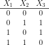
They are certainly not mutually independent because the event  has probability
  , whereas
 ![{\prod_{i=1}^3 {\mathrm{Pr}}[X_i=1]=(1/2)^3}](https://s0.wp.com/latex.php?latex=%7B%5Cprod_%7Bi%3D1%7D%5E3+%7B%5Cmathrm%7BPr%7D%7D%5BX_i%3D1%5D%3D%281%2F2%29%5E3%7D&bg=ffffff&fg=000000&s=0&c=20201002) . But, by checking all cases, one can verify that they are pairwise independent.
. But, by checking all cases, one can verify that they are pairwise independent.
3.1. Constructing Pairwise Independent RVs
Let  be a finite field and
  . We will construct RVs
  such that each
  is uniform over and the ‘s are pairwise independent. To do so, we need to generate only two independent RVs
  and
and  that are uniformly distributed over . We then define

Claim 9 Each is uniformly distributed on .
Proof: For  we have
  , which is uniform. For
  and any
  we have
![\displaystyle \begin{array}{rcl} {\mathrm{Pr}}[ Y_i = j ] &=& {\mathrm{Pr}}[ X_1 + i \cdot X_2 = j ] \\ &=& {\mathrm{Pr}}[ X_2 = (j-X_1)/i ] \\ &=& \sum_{x \in {\mathbb F}} {\mathrm{Pr}}[~ X_2 = (j-x)/i ~\wedge~ X_1=x ~] \qquad(\mathrm{total~probability~law}) \\ &=& \sum_{x \in {\mathbb F}} {\mathrm{Pr}}[ X_2 = (j-x)/i] \cdot {\mathrm{Pr}}[ X_1=x ] \qquad(\mathrm{pairwise~independence}) \\ &=& (1/q) \cdot \sum_{x \in {\mathbb F}} {\mathrm{Pr}}[ X_2 = (j-x)/i ] \\ &=& (1/q), \end{array}](https://s0.wp.com/latex.php?latex=%5Cdisplaystyle+%5Cbegin%7Barray%7D%7Brcl%7D+%7B%5Cmathrm%7BPr%7D%7D%5B+Y_i+%3D+j+%5D+%26%3D%26+%7B%5Cmathrm%7BPr%7D%7D%5B+X_1+%2B+i+%5Ccdot+X_2+%3D+j+%5D+%5C%5C+%26%3D%26+%7B%5Cmathrm%7BPr%7D%7D%5B+X_2+%3D+%28j-X_1%29%2Fi+%5D+%5C%5C+%26%3D%26+%5Csum_%7Bx+%5Cin+%7B%5Cmathbb+F%7D%7D+%7B%5Cmathrm%7BPr%7D%7D%5B%7E+X_2+%3D+%28j-x%29%2Fi+%7E%5Cwedge%7E+X_1%3Dx+%7E%5D+%5Cqquad%28%5Cmathrm%7Btotal%7Eprobability%7Elaw%7D%29+%5C%5C+%26%3D%26+%5Csum_%7Bx+%5Cin+%7B%5Cmathbb+F%7D%7D+%7B%5Cmathrm%7BPr%7D%7D%5B+X_2+%3D+%28j-x%29%2Fi%5D+%5Ccdot+%7B%5Cmathrm%7BPr%7D%7D%5B+X_1%3Dx+%5D+%5Cqquad%28%5Cmathrm%7Bpairwise%7Eindependence%7D%29+%5C%5C+%26%3D%26+%281%2Fq%29+%5Ccdot+%5Csum_%7Bx+%5Cin+%7B%5Cmathbb+F%7D%7D+%7B%5Cmathrm%7BPr%7D%7D%5B+X_2+%3D+%28j-x%29%2Fi+%5D+%5C%5C+%26%3D%26+%281%2Fq%29%2C+%5Cend%7Barray%7D+&bg=ffffff&fg=000000&s=0&c=20201002)
since as  ranges through ,
  also ranges through all of . (In other words, the map
  is a bijection of to itself.) So is uniform.
Claim 10 The ‘s are pairwise independent.
Proof: We wish to show that, for any distinct RVs and  and any values
  , we have
![\displaystyle {\mathrm{Pr}}[~ Y_i=a \:\wedge\: Y_j=b ~] ~=~ {\mathrm{Pr}}[ Y_i=a ] \cdot {\mathrm{Pr}}[ Y_j=b ] ~=~ 1/q^2.](https://s0.wp.com/latex.php?latex=%5Cdisplaystyle+%7B%5Cmathrm%7BPr%7D%7D%5B%7E+Y_i%3Da+%5C%3A%5Cwedge%5C%3A+Y_j%3Db+%7E%5D+%7E%3D%7E+%7B%5Cmathrm%7BPr%7D%7D%5B+Y_i%3Da+%5D+%5Ccdot+%7B%5Cmathrm%7BPr%7D%7D%5B+Y_j%3Db+%5D+%7E%3D%7E+1%2Fq%5E2.+&bg=ffffff&fg=000000&s=0&c=20201002)
This event is equivalent to  and
and  . We can also rewrite that as:

This holds precisely when

Since and are independent and uniform over , this event holds with probability  .
.
Corollary 11 Given  mutually independent, uniformly random bits, we can construct
  pairwise independent, uniformly random strings in
  .
.
Proof: Apply the previous construction to the finite field  . The mutually independent random bits are used to construct and . The random strings
  are constructed as in (1).
3.2. Example: Max Cut with pairwise independent RVs
Once again let’s consider the Max Cut problem. We are given a graph  where
where  . We will choose
  -valued random variables
  . If
. If  then we add vertex to
  .
.
Our original algorithm chose to be mutually independent and uniform. Instead we will pick to be pairwise independent and uniform. Then
![\displaystyle \begin{array}{rcl} {\mathrm E}[ |\delta(U)| ] &=& \sum_{ij \in E} {\mathrm{Pr}}[~ (i \!\in\! U \wedge j \!\not\in\! U) \:\vee\: (i \!\not\in\! U \wedge j \!\in\! U) ~] \\ &=& \sum_{ij \in E} {\mathrm{Pr}}[~ i \!\in\! U \wedge j \!\not\in\! U ~] + {\mathrm{Pr}}[~ i \!\not\in\! U \wedge j \!\in\! U ~] \\ &=& \sum_{ij \in E} {\mathrm{Pr}}[Y_i]{\mathrm{Pr}}[\overline{Y_j}] + {\mathrm{Pr}}[\overline{Y_i}]{\mathrm{Pr}}[Y_j] \qquad(\mathrm{pairwise~independence}) \\ &=& \sum_{ij \in E} \Big( (1/2)^2 + (1/2)^2 \Big) \\ &=& |E|/2 \end{array}](https://s0.wp.com/latex.php?latex=%5Cdisplaystyle+%5Cbegin%7Barray%7D%7Brcl%7D+%7B%5Cmathrm+E%7D%5B+%7C%5Cdelta%28U%29%7C+%5D+%26%3D%26+%5Csum_%7Bij+%5Cin+E%7D+%7B%5Cmathrm%7BPr%7D%7D%5B%7E+%28i+%5C%21%5Cin%5C%21+U+%5Cwedge+j+%5C%21%5Cnot%5Cin%5C%21+U%29+%5C%3A%5Cvee%5C%3A+%28i+%5C%21%5Cnot%5Cin%5C%21+U+%5Cwedge+j+%5C%21%5Cin%5C%21+U%29+%7E%5D+%5C%5C+%26%3D%26+%5Csum_%7Bij+%5Cin+E%7D+%7B%5Cmathrm%7BPr%7D%7D%5B%7E+i+%5C%21%5Cin%5C%21+U+%5Cwedge+j+%5C%21%5Cnot%5Cin%5C%21+U+%7E%5D+%2B+%7B%5Cmathrm%7BPr%7D%7D%5B%7E+i+%5C%21%5Cnot%5Cin%5C%21+U+%5Cwedge+j+%5C%21%5Cin%5C%21+U+%7E%5D+%5C%5C+%26%3D%26+%5Csum_%7Bij+%5Cin+E%7D+%7B%5Cmathrm%7BPr%7D%7D%5BY_i%5D%7B%5Cmathrm%7BPr%7D%7D%5B%5Coverline%7BY_j%7D%5D+%2B+%7B%5Cmathrm%7BPr%7D%7D%5B%5Coverline%7BY_i%7D%5D%7B%5Cmathrm%7BPr%7D%7D%5BY_j%5D+%5Cqquad%28%5Cmathrm%7Bpairwise%7Eindependence%7D%29+%5C%5C+%26%3D%26+%5Csum_%7Bij+%5Cin+E%7D+%5CBig%28+%281%2F2%29%5E2+%2B+%281%2F2%29%5E2+%5CBig%29+%5C%5C+%26%3D%26+%7CE%7C%2F2+%5Cend%7Barray%7D+&bg=ffffff&fg=000000&s=0&c=20201002)
So the original algorithm works just as well if we make pairwise independent decisions instead of mutually independent decisions for placing vertices in . The following theorem shows the advantage of making pairwise independent decisions.
Theorem 12 There is a deterministic, polynomial time algorithm to find a cut  with
with  .
.
Proof: By Corollary 11, we only need  mutually independent, uniform random bits
  in order to generate our pairwise independent, uniform random bits . We have just argued that these pairwise independent ‘s will give us
![\displaystyle {\mathrm E}_{X_1,\ldots,X_b}[ |\delta(U)| ] ~=~ |E|/2.](https://s0.wp.com/latex.php?latex=%5Cdisplaystyle+%7B%5Cmathrm+E%7D_%7BX_1%2C%5Cldots%2CX_b%7D%5B+%7C%5Cdelta%28U%29%7C+%5D+%7E%3D%7E+%7CE%7C%2F2.+&bg=ffffff&fg=000000&s=0&c=20201002)
So there must exist some particular bits  such that fixing
  for all , we get
  . We can deterministically find such bits by exhaustive search in
  trials. This gives a deterministic, polynomial time algorithm.
4. Chebyshev with pairwise independent RVs
One of the main benefits of pairwise independent RVs is that Chebyshev’s inequality still works beautifully. Suppose that are pairwise independent. For any  ,
,
![\displaystyle {\mathrm{Cov}}[X_i,X_j] ~=~ {\mathrm E}[X_i X_j] - {\mathrm E}[X_i]{\mathrm E}[X_j] ~=~ 0,](https://s0.wp.com/latex.php?latex=%5Cdisplaystyle+%7B%5Cmathrm%7BCov%7D%7D%5BX_i%2CX_j%5D+%7E%3D%7E+%7B%5Cmathrm+E%7D%5BX_i+X_j%5D+-+%7B%5Cmathrm+E%7D%5BX_i%5D%7B%5Cmathrm+E%7D%5BX_j%5D+%7E%3D%7E+0%2C+&bg=ffffff&fg=000000&s=0&c=20201002)
by Claim 8. So
![\displaystyle {\mathrm{Var}}[{\textstyle \sum_{i=1}^n X_i}] ~=~ \sum_{i=1}^n {\mathrm{Var}}[X_i],](https://s0.wp.com/latex.php?latex=%5Cdisplaystyle+%7B%5Cmathrm%7BVar%7D%7D%5B%7B%5Ctextstyle+%5Csum_%7Bi%3D1%7D%5En+X_i%7D%5D+%7E%3D%7E+%5Csum_%7Bi%3D1%7D%5En+%7B%5Cmathrm%7BVar%7D%7D%5BX_i%5D%2C+&bg=ffffff&fg=000000&s=0&c=20201002)
by Claim 5. So
![\displaystyle {\mathrm{Pr}}[{\textstyle |\sum_i X_i - {\mathrm E}[\sum_i X_i]| > t }] ~\leq~ \frac{{\mathrm{Var}}[\sum_i X_i]}{t^2}.](https://s0.wp.com/latex.php?latex=%5Cdisplaystyle+%7B%5Cmathrm%7BPr%7D%7D%5B%7B%5Ctextstyle+%7C%5Csum_i+X_i+-+%7B%5Cmathrm+E%7D%5B%5Csum_i+X_i%5D%7C+%3E+t+%7D%5D+%7E%5Cleq%7E+%5Cfrac%7B%7B%5Cmathrm%7BVar%7D%7D%5B%5Csum_i+X_i%5D%7D%7Bt%5E2%7D.+&bg=ffffff&fg=000000&s=0&c=20201002)
This is exactly the same bound that we would get if the ‘s were mutually independent.


.


![{{\mathrm E}[w(T_k)] \leq O(\log n) \cdot c(C^*)}](https://s0.wp.com/latex.php?latex=%7B%7B%5Cmathrm+E%7D%5Bw%28T_k%29%5D+%5Cleq+O%28%5Clog+n%29+%5Ccdot+c%28C%5E%2A%29%7D&bg=ffffff&fg=000000&s=0&c=20201002)
![{\pi : [k] \rightarrow U}](https://s0.wp.com/latex.php?latex=%7B%5Cpi+%3A+%5Bk%5D+%5Crightarrow+U%7D&bg=ffffff&fg=000000&s=0&c=20201002)


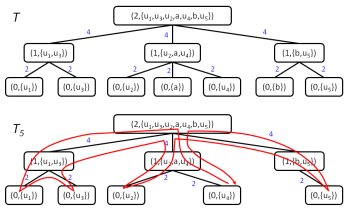

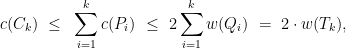
![\displaystyle {\mathrm E}[\, w(T_k) \,] ~\leq~ {\mathrm E}\Big[\: \sum_{i=1}^k d_T(\pi_i,\pi_{i+1}) \:\Big] \\ ~\leq~ O(\log n) \cdot \sum_{i=1}^k d_G(\pi_i,\pi_{i+1}) \\ ~\leq~ O(\log n) \cdot c(C^*), \ \ \ \ \ (3)](https://s0.wp.com/latex.php?latex=%5Cdisplaystyle+%7B%5Cmathrm+E%7D%5B%5C%2C+w%28T_k%29+%5C%2C%5D+%7E%5Cleq%7E+%7B%5Cmathrm+E%7D%5CBig%5B%5C%3A+%5Csum_%7Bi%3D1%7D%5Ek+d_T%28%5Cpi_i%2C%5Cpi_%7Bi%2B1%7D%29+%5C%3A%5CBig%5D+%5C%5C+%7E%5Cleq%7E+O%28%5Clog+n%29+%5Ccdot+%5Csum_%7Bi%3D1%7D%5Ek+d_G%28%5Cpi_i%2C%5Cpi_%7Bi%2B1%7D%29+%5C%5C+%7E%5Cleq%7E+O%28%5Clog+n%29+%5Ccdot+c%28C%5E%2A%29%2C+%5C+%5C+%5C+%5C+%5C+%283%29&bg=ffffff&fg=000000&s=0&c=20201002)

![{{\mathrm E}[ d_T(\pi_i,\pi_{i+1}) ]}](https://s0.wp.com/latex.php?latex=%7B%7B%5Cmathrm+E%7D%5B+d_T%28%5Cpi_i%2C%5Cpi_%7Bi%2B1%7D%29+%5D%7D&bg=ffffff&fg=000000&s=0&c=20201002)

![{{\mathrm E}[w(T_k)]}](https://s0.wp.com/latex.php?latex=%7B%7B%5Cmathrm+E%7D%5Bw%28T_k%29%5D%7D&bg=ffffff&fg=000000&s=0&c=20201002)

be the closest vertex to
amongst
, using distances in
.
be a shortest path in
.

be the unique path in
.
.

 for all


![\displaystyle {\mathrm E}[ c(C_k) ] ~\leq~ O(\log n) \cdot c(C^*),](https://s0.wp.com/latex.php?latex=%5Cdisplaystyle+%7B%5Cmathrm+E%7D%5B+c%28C_k%29+%5D+%7E%5Cleq%7E+O%28%5Clog+n%29+%5Ccdot+c%28C%5E%2A%29%2C+&bg=ffffff&fg=000000&s=0&c=20201002)
 be an edge and let
  be the corresponding tree. Is the shortest path metric of
  and
and  , whereas the distance between
  . So, no matter which subtree
  (possibly with lengths on the edges) where
  and
and  is completely unrelated to
  . Can such a tree do a better job of approximating distances in
  . But here is a small observation: any subtree of
  , for both
  . Let
. Let  be the distance between
  at random and let
  be the
  since we constructed
 ![{{\mathrm E}[ d_T(u,v) ]}](https://s0.wp.com/latex.php?latex=%7B%7B%5Cmathrm+E%7D%5B+d_T%28u%2Cv%29+%5D%7D&bg=ffffff&fg=000000&s=0&c=20201002) . If
. If  ; the probability of that happening is
  . Otherwise,
  . Thus,
![\displaystyle {\mathrm E}[ d_T(u,v) ] ~=~ (d/n) \cdot (n-d) + (1-d/n) \cdot d ~\leq~ 2d.](https://s0.wp.com/latex.php?latex=%5Cdisplaystyle+%7B%5Cmathrm+E%7D%5B+d_T%28u%2Cv%29+%5D+%7E%3D%7E+%28d%2Fn%29+%5Ccdot+%28n-d%29+%2B+%281-d%2Fn%29+%5Ccdot+d+%7E%5Cleq%7E+2d.+&bg=ffffff&fg=000000&s=0&c=20201002)
 with
with  , there is an algorithm that generates a random tree for which all distances are approximated to within a factor of
  , a tree
  , and weights
  such that
![\displaystyle {\mathrm E}[ d_T\big(f(x),f(y)\big) ] ~\leq~ O(\log n) \cdot d_X(x,y) \quad\forall x,y \in X. \ \ \ \ \ (2)](https://s0.wp.com/latex.php?latex=%5Cdisplaystyle+%7B%5Cmathrm+E%7D%5B+d_T%5Cbig%28f%28x%29%2Cf%28y%29%5Cbig%29+%5D+%7E%5Cleq%7E+O%28%5Clog+n%29+%5Ccdot+d_X%28x%2Cy%29+%5Cquad%5Cforall+x%2Cy+%5Cin+X.+%5C+%5C+%5C+%5C+%5C+%282%29&bg=ffffff&fg=000000&s=0&c=20201002)
 such that such that
  for all distinct
  . Note that
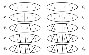
  -bounded random partition
  of
of  then assemble those partitions into the desired tree. Assembling them is not too difficult, but there is one annoyance: the parts of
  for any
  . If the parts of
  then this would induce a natural hierarchy on the parts, and therefore give us a nice tree structure.
 , for
, for 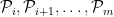 . In
. In 
 is the meet operation in the partition lattice. If you’re not familiar with this notation, don’t worry; it is easy to explain. Simply define
  , then let
 , so we have obtained the desired hierarchical structure.
 for the points
  , and the corresponding partitions
  .
.

 : The vertices in
  where
where  and
and  . The vertices and edges of the tree
  as the root of the tree.
 downto
  .
. , add the vertex
  to
to  , connected by an edge of length
  .
.  for all distinct
  and since
  is
is  . 1.5. Analysis
  . Let
. Let  be the largest index with
  . Then
  .
.  is the highest level of the
  are separated. A simple inductive argument shows that
  and
and  is at level
  . Let us call the least common ancestor
 , the proof is complete.
  . Since
  . By Claim
 . We have
![\displaystyle \begin{array}{rcl} {\mathrm E}[\: d_T\big(f(x),f(y)\big) \:] &=& \sum_{i=0}^m {\mathrm{Pr}}[\: i \mathrm{~is~the~largest~index~with~} {\mathcal P}_i(x) \neq {\mathcal P}_i(y) \:] \cdot (2^{i+3} - 4) \\ &<& \sum_{i=0}^m {\mathrm{Pr}}[ {\mathcal P}_i(x) \neq {\mathcal P}_i(y) ] \cdot 2^{i+3} \\ &\leq& \sum_{i=0}^m {\mathrm{Pr}}[ B(x,r) \not\subseteq {\mathcal P}_i(x) ] \cdot 2^{i+3} \\ &\leq& O(\log n) \cdot r, \end{array}](https://s0.wp.com/latex.php?latex=%5Cdisplaystyle+%5Cbegin%7Barray%7D%7Brcl%7D+%7B%5Cmathrm+E%7D%5B%5C%3A+d_T%5Cbig%28f%28x%29%2Cf%28y%29%5Cbig%29+%5C%3A%5D+%26%3D%26+%5Csum_%7Bi%3D0%7D%5Em+%7B%5Cmathrm%7BPr%7D%7D%5B%5C%3A+i+%5Cmathrm%7B%7Eis%7Ethe%7Elargest%7Eindex%7Ewith%7E%7D+%7B%5Cmathcal+P%7D_i%28x%29+%5Cneq+%7B%5Cmathcal+P%7D_i%28y%29+%5C%3A%5D+%5Ccdot+%282%5E%7Bi%2B3%7D+-+4%29+%5C%5C+%26%3C%26+%5Csum_%7Bi%3D0%7D%5Em+%7B%5Cmathrm%7BPr%7D%7D%5B+%7B%5Cmathcal+P%7D_i%28x%29+%5Cneq+%7B%5Cmathcal+P%7D_i%28y%29+%5D+%5Ccdot+2%5E%7Bi%2B3%7D+%5C%5C+%26%5Cleq%26+%5Csum_%7Bi%3D0%7D%5Em+%7B%5Cmathrm%7BPr%7D%7D%5B+B%28x%2Cr%29+%5Cnot%5Csubseteq+%7B%5Cmathcal+P%7D_i%28x%29+%5D+%5Ccdot+2%5E%7Bi%2B3%7D+%5C%5C+%26%5Cleq%26+O%28%5Clog+n%29+%5Ccdot+r%2C+%5Cend%7Barray%7D+&bg=ffffff&fg=000000&s=0&c=20201002)
 and
and  ,
,![\displaystyle \sum_{i=0}^m {\mathrm{Pr}}[ B(x,r) \not\subseteq {\mathcal P}_i(x) ] \cdot 2^{i+3} ~\leq~ O(\log n) \cdot r.](https://s0.wp.com/latex.php?latex=%5Cdisplaystyle+%5Csum_%7Bi%3D0%7D%5Em+%7B%5Cmathrm%7BPr%7D%7D%5B+B%28x%2Cr%29+%5Cnot%5Csubseteq+%7B%5Cmathcal+P%7D_i%28x%29+%5D+%5Ccdot+2%5E%7Bi%2B3%7D+%7E%5Cleq%7E+O%28%5Clog+n%29+%5Ccdot+r.+&bg=ffffff&fg=000000&s=0&c=20201002)
 . Then
![\displaystyle \begin{array}{rcl} & & \sum_{i=0}^m {\mathrm{Pr}}[ B(x,r) \not\subseteq {\mathcal P}_i(x) ] \cdot 2^{i+3} \\ &\leq& \sum_{i=0}^{k+3} 2^{i+3} ~+~ \sum_{i=k+4}^m \frac{8r}{2^i} \cdot H\Big( |B(x,2^{i-2}-r)|, |B(x,2^{i-1}+r)| \Big) \cdot 2^{i+3} \\ &\leq& 128r ~+~ 64r \cdot \sum_{i=k+4}^m H\Big( |B(x,2^{i-3})|, |B(x,2^i)| \Big), \end{array}](https://s0.wp.com/latex.php?latex=%5Cdisplaystyle+%5Cbegin%7Barray%7D%7Brcl%7D+%26+%26+%5Csum_%7Bi%3D0%7D%5Em+%7B%5Cmathrm%7BPr%7D%7D%5B+B%28x%2Cr%29+%5Cnot%5Csubseteq+%7B%5Cmathcal+P%7D_i%28x%29+%5D+%5Ccdot+2%5E%7Bi%2B3%7D+%5C%5C+%26%5Cleq%26+%5Csum_%7Bi%3D0%7D%5E%7Bk%2B3%7D+2%5E%7Bi%2B3%7D+%7E%2B%7E+%5Csum_%7Bi%3Dk%2B4%7D%5Em+%5Cfrac%7B8r%7D%7B2%5Ei%7D+%5Ccdot+H%5CBig%28+%7CB%28x%2C2%5E%7Bi-2%7D-r%29%7C%2C+%7CB%28x%2C2%5E%7Bi-1%7D%2Br%29%7C+%5CBig%29+%5Ccdot+2%5E%7Bi%2B3%7D+%5C%5C+%26%5Cleq%26+128r+%7E%2B%7E+64r+%5Ccdot+%5Csum_%7Bi%3Dk%2B4%7D%5Em+H%5CBig%28+%7CB%28x%2C2%5E%7Bi-3%7D%29%7C%2C+%7CB%28x%2C2%5Ei%29%7C+%5CBig%29%2C+%5Cend%7Barray%7D+&bg=ffffff&fg=000000&s=0&c=20201002)
 when
when  . The final sum is upper bounded as follows.
 . Let
. Let  be the ball of radius
  around
  , there is
  -bounded random partition
  of
of ![\displaystyle {\mathrm{Pr}}[ B(x,r) \not\subseteq {\mathcal P}(x) ] ~\leq~ \frac{ 8r }{ \Delta } \:\cdot\: H\big(\: |B(x,\Delta/4-r)|,\: |B(x,\Delta/2+r)| \:\big) \quad \forall x \in X ,\: \forall r>0. \ \ \ \ \ (1)](https://s0.wp.com/latex.php?latex=%5Cdisplaystyle+%7B%5Cmathrm%7BPr%7D%7D%5B+B%28x%2Cr%29+%5Cnot%5Csubseteq+%7B%5Cmathcal+P%7D%28x%29+%5D+%7E%5Cleq%7E+%5Cfrac%7B+8r+%7D%7B+%5CDelta+%7D+%5C%3A%5Ccdot%5C%3A+H%5Cbig%28%5C%3A+%7CB%28x%2C%5CDelta%2F4-r%29%7C%2C%5C%3A+%7CB%28x%2C%5CDelta%2F2%2Br%29%7C+%5C%3A%5Cbig%29+%5Cquad+%5Cforall+x+%5Cin+X+%2C%5C%3A+%5Cforall+r%3E0.+%5C+%5C+%5C+%5C+%5C+%281%29&bg=ffffff&fg=000000&s=0&c=20201002)
![{\alpha \in (1/4,1/2]}](https://s0.wp.com/latex.php?latex=%7B%5Calpha+%5Cin+%281%2F4%2C1%2F2%5D%7D&bg=ffffff&fg=000000&s=0&c=20201002) uniformly at random.
uniformly at random. uniformly at random.
 .
. .We have already proven that this outputs a
  . For brevity let
  . Let us order all points of
  where
where  . The proof involves two important definitions.
 if
if  .
. .
. and
and  is the Euclidean metric. Then
  intersects
  .
. .
. .
. and
and  both see
  does not. The point
 .
. iterations of the algorithm did not assign any point in
  do not see
  . Consequently
 . Thus
 . Since
  , we have shown that
![\displaystyle {\mathrm{Pr}}[ B \not\subseteq {\mathcal P}(x) ] ~\leq~ {\mathrm{Pr}}[ y_{\pi(k)} \mathrm{~cuts~} B ] ~=~ \sum_{i=1}^n {\mathrm{Pr}}[ y_{\pi(k)}=y_i ~\wedge~ y_i \mathrm{~cuts~} B ].](https://s0.wp.com/latex.php?latex=%5Cdisplaystyle+%7B%5Cmathrm%7BPr%7D%7D%5B+B+%5Cnot%5Csubseteq+%7B%5Cmathcal+P%7D%28x%29+%5D+%7E%5Cleq%7E+%7B%5Cmathrm%7BPr%7D%7D%5B+y_%7B%5Cpi%28k%29%7D+%5Cmathrm%7B%7Ecuts%7E%7D+B+%5D+%7E%3D%7E+%5Csum_%7Bi%3D1%7D%5En+%7B%5Cmathrm%7BPr%7D%7D%5B+y_%7B%5Cpi%28k%29%7D%3Dy_i+%7E%5Cwedge%7E+y_i+%5Cmathrm%7B%7Ecuts%7E%7D+B+%5D.+&bg=ffffff&fg=000000&s=0&c=20201002)
 then
then  then
then  and
and  . Then we have shown that
![\displaystyle {\mathrm{Pr}}[ B \not\subseteq {\mathcal P}(x) ] ~\leq~ \sum_{i=a+1}^b {\mathrm{Pr}}[ y_{\pi(k)}=y_i ~\wedge~ y_i \mathrm{~cuts~} B ].](https://s0.wp.com/latex.php?latex=%5Cdisplaystyle+%7B%5Cmathrm%7BPr%7D%7D%5B+B+%5Cnot%5Csubseteq+%7B%5Cmathcal+P%7D%28x%29+%5D+%7E%5Cleq%7E+%5Csum_%7Bi%3Da%2B1%7D%5Eb+%7B%5Cmathrm%7BPr%7D%7D%5B+y_%7B%5Cpi%28k%29%7D%3Dy_i+%7E%5Cwedge%7E+y_i+%5Cmathrm%7B%7Ecuts%7E%7D+B+%5D.+&bg=ffffff&fg=000000&s=0&c=20201002)
 and
and  ” depends only on
  ” depends primarily on
 ![\displaystyle {\mathrm{Pr}}[ B \not\subseteq {\mathcal P}(x) ] ~\leq~ \sum_{i=a+1}^b {\mathrm{Pr}}[ y_i \mathrm{~cuts~} B ] \cdot {\mathrm{Pr}}[\: y_{\pi(k)}=y_i \:|\: y_i \mathrm{~cuts~} B ]](https://s0.wp.com/latex.php?latex=%5Cdisplaystyle+%7B%5Cmathrm%7BPr%7D%7D%5B+B+%5Cnot%5Csubseteq+%7B%5Cmathcal+P%7D%28x%29+%5D+%7E%5Cleq%7E+%5Csum_%7Bi%3Da%2B1%7D%5Eb+%7B%5Cmathrm%7BPr%7D%7D%5B+y_i+%5Cmathrm%7B%7Ecuts%7E%7D+B+%5D+%5Ccdot+%7B%5Cmathrm%7BPr%7D%7D%5B%5C%3A+y_%7B%5Cpi%28k%29%7D%3Dy_i+%5C%3A%7C%5C%3A+y_i+%5Cmathrm%7B%7Ecuts%7E%7D+B+%5D+&bg=ffffff&fg=000000&s=0&c=20201002)
![\displaystyle {\mathrm{Pr}}[ y_i \mathrm{~cuts~} B ] ~=~ {\mathrm{Pr}}[\: \alpha \Delta \in [d(x,y)-r,d(x,y)+r] \:] ~\leq~ \frac{2r}{\Delta/4},](https://s0.wp.com/latex.php?latex=%5Cdisplaystyle+%7B%5Cmathrm%7BPr%7D%7D%5B+y_i+%5Cmathrm%7B%7Ecuts%7E%7D+B+%5D+%7E%3D%7E+%7B%5Cmathrm%7BPr%7D%7D%5B%5C%3A+%5Calpha+%5CDelta+%5Cin+%5Bd%28x%2Cy%29-r%2Cd%28x%2Cy%29%2Br%5D+%5C%3A%5D+%7E%5Cleq%7E+%5Cfrac%7B2r%7D%7B%5CDelta%2F4%7D%2C+&bg=ffffff&fg=000000&s=0&c=20201002)
 is the length of the interval
 ![{[d(x,y)-r,d(x,y)+r]}](https://s0.wp.com/latex.php?latex=%7B%5Bd%28x%2Cy%29-r%2Cd%28x%2Cy%29%2Br%5D%7D&bg=ffffff&fg=000000&s=0&c=20201002) and
and  is the length of the interval from which
  is randomly chosen.
 cuts
cuts  . Every
  coming earlier in the ordering has
  , so
, so  .
.![\displaystyle {\mathrm{Pr}}[ B \not\subseteq {\mathcal P}(x) ] ~\leq~ \sum_{i=a+1}^b \frac{8r}{\Delta} \cdot \frac{1}{i} ~=~ \frac{8r}{\Delta} \cdot H(a,b),](https://s0.wp.com/latex.php?latex=%5Cdisplaystyle+%7B%5Cmathrm%7BPr%7D%7D%5B+B+%5Cnot%5Csubseteq+%7B%5Cmathcal+P%7D%28x%29+%5D+%7E%5Cleq%7E+%5Csum_%7Bi%3Da%2B1%7D%5Eb+%5Cfrac%7B8r%7D%7B%5CDelta%7D+%5Ccdot+%5Cfrac%7B1%7D%7Bi%7D+%7E%3D%7E+%5Cfrac%7B8r%7D%7B%5CDelta%7D+%5Ccdot+H%28a%2Cb%29%2C+&bg=ffffff&fg=000000&s=0&c=20201002)
 such that every metric has a
  -bounded,
  -Lipschitz random partition. We now show that this is optimal.
 .
.  and
and  :
: for all
  .
. ,
,  and
and  . (The constant
  can of course be improved.)
 that is
  -regular, the number of vertices in
  . So every part
  . By the expansion condition, the number of edges cut is at least
 . Every point
  has
has  , so
, so  , implying that
  .
. . Every point
  , implying that
  .
.  , which is at least
  . So
. So  , implying that
  , which is strictly less than
  . So
. So  such that
 for all
  for all
  for
for  ).
). for all
  for all
  .
. .
. ) Metric:
  and
and  .
. ) Metric:
  .
. . The distance function is defined by letting
  be the length of the shortest path between
  and keeping the same distance functions. In computer science we are often only interested in finite metric spaces because the input data to the problem is finite.
 be a partition of
  be the unique part
  . We say that the partition
 ![\displaystyle {\mathrm{Pr}}[ {\mathcal P}(x) \neq {\mathcal P}(y) ] ~\leq~ L \cdot d(x,y) \qquad \forall x,y \in X.](https://s0.wp.com/latex.php?latex=%5Cdisplaystyle+%7B%5Cmathrm%7BPr%7D%7D%5B+%7B%5Cmathcal+P%7D%28x%29+%5Cneq+%7B%5Cmathcal+P%7D%28y%29+%5D+%7E%5Cleq%7E+L+%5Ccdot+d%28x%2Cy%29+%5Cqquad+%5Cforall+x%2Cy+%5Cin+X.+&bg=ffffff&fg=000000&s=0&c=20201002)
 ,
,  . The diameter of this metric is clearly
  and
and  . This partition is
  . Does it capture our goal that “close points should end up in the same part”?
 and
and  , so most pairs of consecutive points did end up in the same part. But if we modify our metric slightly, this is no longer true. Consider making
  uniformly at random, then set
  and
and  . Let
. Let  (even if we made multiple copies of points). So
  .
. . They end up in different parts of the partition only if
  , which happens with probability at most
  . Thus
 ![{{\mathrm{Pr}}[ {\mathcal P}(i) \neq {\mathcal P}(i+1) ] \leq 3/n}](https://s0.wp.com/latex.php?latex=%7B%7B%5Cmathrm%7BPr%7D%7D%5B+%7B%5Cmathcal+P%7D%28i%29+%5Cneq+%7B%5Cmathcal+P%7D%28i%2B1%29+%5D+%5Cleq+3%2Fn%7D&bg=ffffff&fg=000000&s=0&c=20201002) . More generally
. More generally![\displaystyle {\mathrm{Pr}}[ {\mathcal P}(x) \neq {\mathcal P}(y) ] ~\leq~ \frac{3}{n} \cdot d(x,y).](https://s0.wp.com/latex.php?latex=%5Cdisplaystyle+%7B%5Cmathrm%7BPr%7D%7D%5B+%7B%5Cmathcal+P%7D%28x%29+%5Cneq+%7B%5Cmathcal+P%7D%28y%29+%5D+%7E%5Cleq%7E+%5Cfrac%7B3%7D%7Bn%7D+%5Ccdot+d%28x%2Cy%29.+&bg=ffffff&fg=000000&s=0&c=20201002)
 . The key point is: this holds regardless of how many copies of the points we make. So this same random partition
  . We can think of this as meaning that the probability of adjacent points ending up in different parts is roughly the inverse of the diameter of those parts. Our main theorem is that, by increasing
  .
.  .
.![\displaystyle {\mathrm{Pr}}[ B(x,r) \not\subseteq {\mathcal P}(x) ] ~\leq~ \frac{8r}{\Delta} \:\cdot\: H\big(\: |B(x,\Delta/4-r)|,\: |B(x,\Delta/2+r)| \:\big) \qquad \forall x \in X ,\: \forall r>0. \ \ \ \ \ (1)](https://s0.wp.com/latex.php?latex=%5Cdisplaystyle+%7B%5Cmathrm%7BPr%7D%7D%5B+B%28x%2Cr%29+%5Cnot%5Csubseteq+%7B%5Cmathcal+P%7D%28x%29+%5D+%7E%5Cleq%7E+%5Cfrac%7B8r%7D%7B%5CDelta%7D+%5C%3A%5Ccdot%5C%3A+H%5Cbig%28%5C%3A+%7CB%28x%2C%5CDelta%2F4-r%29%7C%2C%5C%3A+%7CB%28x%2C%5CDelta%2F2%2Br%29%7C+%5C%3A%5Cbig%29+%5Cqquad+%5Cforall+x+%5Cin+X+%2C%5C%3A+%5Cforall+r%3E0.+%5C+%5C+%5C+%5C+%5C+%281%29&bg=ffffff&fg=000000&s=0&c=20201002)
 . Note that if
  . Thus
![\displaystyle \begin{array}{rcl} {\mathrm{Pr}}[ {\mathcal P}(x) \neq {\mathcal P}(y) ] &\leq& (8r/\Delta) \cdot H\big(\: |B(x,\Delta/4-r)|,\: |B(x,\Delta/2+r)| \:\big) \\ &\leq& (8r/\Delta) \cdot H(0, n ) \\ &=& O(\log(n)/\Delta) \cdot d(x,y), \end{array}](https://s0.wp.com/latex.php?latex=%5Cdisplaystyle+%5Cbegin%7Barray%7D%7Brcl%7D+%7B%5Cmathrm%7BPr%7D%7D%5B+%7B%5Cmathcal+P%7D%28x%29+%5Cneq+%7B%5Cmathcal+P%7D%28y%29+%5D+%26%5Cleq%26+%288r%2F%5CDelta%29+%5Ccdot+H%5Cbig%28%5C%3A+%7CB%28x%2C%5CDelta%2F4-r%29%7C%2C%5C%3A+%7CB%28x%2C%5CDelta%2F2%2Br%29%7C+%5C%3A%5Cbig%29+%5C%5C+%26%5Cleq%26+%288r%2F%5CDelta%29+%5Ccdot+H%280%2C+n+%29+%5C%5C+%26%3D%26+O%28%5Clog%28n%29%2F%5CDelta%29+%5Ccdot+d%28x%2Cy%29%2C+%5Cend%7Barray%7D+&bg=ffffff&fg=000000&s=0&c=20201002)
 .
.  with
with  , so the
  is either contained in
  , the diameter of
  .
. is not chopped into pieces by the partition. But the parts of the partition are themselves balls of radius at least
  , we might be optimistic that the ball
  . The algorithm generates the following partition.
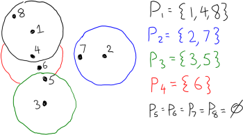
 , decide if it is either a linear function or far from a linear function. There is a property testing algorithm for this problem that uses only a constant number of queries. This algorithm is a key ingredient in proving the infamous
  be a list of
  numbers for the remaining list to be sorted”. In other words, we wish to distinguish the following two scenarios:
 .
. .
. entries of the list.
 . Consider the input
 , which happens with low probability.
 uniformly at random.
 in the list using binary search.
 with
with  . Let
. Let  , which implies that
  by distinctness.
 .
.  ,
,  and maximum degree
  .
. be an arbitrary bijection.
 .
. .
.  in time
  .
.  .
. .
.
 if
if  .
. and
and ![{\mu = {\mathrm E}[X]}](https://s0.wp.com/latex.php?latex=%7B%5Cmu+%3D+%7B%5Cmathrm+E%7D%5BX%5D%7D&bg=ffffff&fg=000000&s=0&c=20201002) . The actual number of edges in
. The actual number of edges in ![\displaystyle |M| ~=~ {\mathrm E}[X_i] m ~=~ {\textstyle \frac{m}{k} \mu}.](https://s0.wp.com/latex.php?latex=%5Cdisplaystyle+%7CM%7C+%7E%3D%7E+%7B%5Cmathrm+E%7D%5BX_i%5D+m+%7E%3D%7E+%7B%5Ctextstyle+%5Cfrac%7Bm%7D%7Bk%7D+%5Cmu%7D.+&bg=ffffff&fg=000000&s=0&c=20201002)
 . Since
  , Fact
 ![{{\mathrm E}[X_i] \geq 1/d^2}](https://s0.wp.com/latex.php?latex=%7B%7B%5Cmathrm+E%7D%5BX_i%5D+%5Cgeq+1%2Fd%5E2%7D&bg=ffffff&fg=000000&s=0&c=20201002) , which implies that
, which implies that  . Therefore
![\displaystyle \begin{array}{rcl} {\textstyle {\mathrm{Pr}}\Big[~ (1-\epsilon) \frac{m}{k} \mu \leq \frac{m}{k} X \leq (1+\epsilon) \frac{m}{k} \mu ~\Big] } &=& {\mathrm{Pr}}\Big[~ (1-\epsilon) \mu \leq X \leq (1+\epsilon) \mu ~\Big] \\ &\geq& 1-2\exp(-\epsilon^2 \mu / 3) ~\geq~ 0.9, \end{array}](https://s0.wp.com/latex.php?latex=%5Cdisplaystyle+%5Cbegin%7Barray%7D%7Brcl%7D+%7B%5Ctextstyle+%7B%5Cmathrm%7BPr%7D%7D%5CBig%5B%7E+%281-%5Cepsilon%29+%5Cfrac%7Bm%7D%7Bk%7D+%5Cmu+%5Cleq+%5Cfrac%7Bm%7D%7Bk%7D+X+%5Cleq+%281%2B%5Cepsilon%29+%5Cfrac%7Bm%7D%7Bk%7D+%5Cmu+%7E%5CBig%5D+%7D+%26%3D%26+%7B%5Cmathrm%7BPr%7D%7D%5CBig%5B%7E+%281-%5Cepsilon%29+%5Cmu+%5Cleq+X+%5Cleq+%281%2B%5Cepsilon%29+%5Cmu+%7E%5CBig%5D+%5C%5C+%26%5Cgeq%26+1-2%5Cexp%28-%5Cepsilon%5E2+%5Cmu+%2F+3%29+%7E%5Cgeq%7E+0.9%2C+%5Cend%7Barray%7D+&bg=ffffff&fg=000000&s=0&c=20201002)
![{r_e \in [0,1]}](https://s0.wp.com/latex.php?latex=%7Br_e+%5Cin+%5B0%2C1%5D%7D&bg=ffffff&fg=000000&s=0&c=20201002) with each edge
with each edge  . They are all distinct with probability
  sharing an endpoint with
  , recursively test if
  is in the matching. If so, return “No”.
 is equivalent to the greedy algorithm. The only question is: what is the running time of the oracle?
 reachable by a path of length
  values in decreasing order. The probability of that event is
  . The number of edges reachable by a path of length
  . So the expected number of nodes explored is less than
  . So the expected time required by an oracle call is
  .
. times, the expected total running time is
  be a bipartite graph, where
  is the set of right-vertices, and
  , let
, let
 -expander if
  ,
,  , every vertex in
 , there exists an
  but it is interesting even in the case
  .
. , we randomly choose exactly
  . We need to show that
  . We do this in a very naive way. We simply consider every set
  with
with  and show that it is unlikely that
  . That probability is easy to analyze:
![\displaystyle {\mathrm{Pr}}[ \Gamma(S) \subseteq T ] ~=~ \Big( \frac{|T|}{m} \Big)^{|S|d}.](https://s0.wp.com/latex.php?latex=%5Cdisplaystyle+%7B%5Cmathrm%7BPr%7D%7D%5B+%5CGamma%28S%29+%5Csubseteq+T+%5D+%7E%3D%7E+%5CBig%28+%5Cfrac%7B%7CT%7C%7D%7Bm%7D+%5CBig%29%5E%7B%7CS%7Cd%7D.+&bg=ffffff&fg=000000&s=0&c=20201002)
 . (In fact, we will simplify our notation by considering the negligibly harder case of
  .) As long as
  is not contained in any such
  and
and ![\displaystyle \begin{array}{rcl} {\mathrm{Pr}}[ G \mathrm{~is~not~a~} (n,m,d)-\mathrm{expander} ] &\leq& \sum_{\substack{S \subseteq L \\ |S| \leq n/2}} ~ \sum_{\substack{T \subseteq R \\ |T|=|S|}} {\mathrm{Pr}}[ \Gamma(S) \subseteq T ] \\ &\leq& \sum_{s \leq n/2} \binom{n}{s} \binom{m}{s} (s/m)^{sd} \\ &\leq& \sum_{s \leq n/2} \Big( \frac{ne}{s} \Big)^s \Big(\frac{me}{s}\Big)^s \Big(\frac{s}{m}\Big)^{sd} \\ &\leq& \sum_{s \leq n/2} \Bigg( \frac{ne}{m} \frac{me}{m} \frac{s^{d-2}}{m^{d-2}}\Bigg)^{s} \\ &\leq& \sum_{s \leq n/2} \Bigg( \frac{ne^2}{(7/8)n} \frac{(n/2)^{d-2}}{\big((7/8)n\big)^{d-2}}\Bigg)^{s} \\ &\leq& \sum_{s \leq n/2} \Bigg( \frac{8e^2}{7} (4/7)^{d-2} \Bigg)^{s} \\ &\leq& \sum_{s=1}^{\infty} \Bigg( 8.5 \cdot 0.58^{d-2} \Bigg)^{s}. \end{array}](https://s0.wp.com/latex.php?latex=%5Cdisplaystyle+%5Cbegin%7Barray%7D%7Brcl%7D+%7B%5Cmathrm%7BPr%7D%7D%5B+G+%5Cmathrm%7B%7Eis%7Enot%7Ea%7E%7D+%28n%2Cm%2Cd%29-%5Cmathrm%7Bexpander%7D+%5D+%26%5Cleq%26+%5Csum_%7B%5Csubstack%7BS+%5Csubseteq+L+%5C%5C+%7CS%7C+%5Cleq+n%2F2%7D%7D+%7E+%5Csum_%7B%5Csubstack%7BT+%5Csubseteq+R+%5C%5C+%7CT%7C%3D%7CS%7C%7D%7D+%7B%5Cmathrm%7BPr%7D%7D%5B+%5CGamma%28S%29+%5Csubseteq+T+%5D+%5C%5C+%26%5Cleq%26+%5Csum_%7Bs+%5Cleq+n%2F2%7D+%5Cbinom%7Bn%7D%7Bs%7D+%5Cbinom%7Bm%7D%7Bs%7D+%28s%2Fm%29%5E%7Bsd%7D+%5C%5C+%26%5Cleq%26+%5Csum_%7Bs+%5Cleq+n%2F2%7D+%5CBig%28+%5Cfrac%7Bne%7D%7Bs%7D+%5CBig%29%5Es+%5CBig%28%5Cfrac%7Bme%7D%7Bs%7D%5CBig%29%5Es+%5CBig%28%5Cfrac%7Bs%7D%7Bm%7D%5CBig%29%5E%7Bsd%7D+%5C%5C+%26%5Cleq%26+%5Csum_%7Bs+%5Cleq+n%2F2%7D+%5CBigg%28+%5Cfrac%7Bne%7D%7Bm%7D+%5Cfrac%7Bme%7D%7Bm%7D+%5Cfrac%7Bs%5E%7Bd-2%7D%7D%7Bm%5E%7Bd-2%7D%7D%5CBigg%29%5E%7Bs%7D+%5C%5C+%26%5Cleq%26+%5Csum_%7Bs+%5Cleq+n%2F2%7D+%5CBigg%28+%5Cfrac%7Bne%5E2%7D%7B%287%2F8%29n%7D+%5Cfrac%7B%28n%2F2%29%5E%7Bd-2%7D%7D%7B%5Cbig%28%287%2F8%29n%5Cbig%29%5E%7Bd-2%7D%7D%5CBigg%29%5E%7Bs%7D+%5C%5C+%26%5Cleq%26+%5Csum_%7Bs+%5Cleq+n%2F2%7D+%5CBigg%28+%5Cfrac%7B8e%5E2%7D%7B7%7D+%284%2F7%29%5E%7Bd-2%7D+%5CBigg%29%5E%7Bs%7D+%5C%5C+%26%5Cleq%26+%5Csum_%7Bs%3D1%7D%5E%7B%5Cinfty%7D+%5CBigg%28+8.5+%5Ccdot+0.58%5E%7Bd-2%7D+%5CBigg%29%5E%7Bs%7D.+%5Cend%7Barray%7D+&bg=ffffff&fg=000000&s=0&c=20201002)
 , the base of the exponent is less than
  , and so the infinite series adds up to less than
  .
. and
and  with
with  . The vertices in
  are called the inputs and the vertices in
  are called the outputs. The graph
  and every
  and
and  with
with  , there are
  has to arrive at a particular
  ; it is acceptable for it to arrive at an arbitrary
  but we do not care what that mapping is.
 edges: simply add an edge between every vertex in
  edges are necessary. His conjecture came from an attempt to prove a lower bound in circuit complexity. But a short while later he realized that his own conjecture was false:
 edges.
  be a
be a  -expander. For every set
  , there is a matching in
  covering
  such that
  for every
  has
has  . That condition holds by
  and
and  with
with  .
. be the number of edges used in a superconcentrator on
  edges for each of the two expanders.
 edges for the smaller superconcentrator.
 . For the base case, we can take
  whenever
  .
. . By Claim
  be the other endpoints of that matching. Similarly, the second expander contains a matching covering
  be the other endpoints of that matching. Note that
  . By induction, the smaller superconcentrator contains
  and
and  . Combining those paths with the edges of the matchings gives the desired paths between
  . Claim
  vertices in
 ![\displaystyle {\mathrm{Pr}}[\: \wedge_{i=1}^n \overline{{\mathcal E}_i} \:] ~=~ \prod_{i=1}^n {\mathrm{Pr}}[ \overline{{\mathcal E}_i} ] ~>~ 0](https://s0.wp.com/latex.php?latex=%5Cdisplaystyle+%7B%5Cmathrm%7BPr%7D%7D%5B%5C%3A+%5Cwedge_%7Bi%3D1%7D%5En+%5Coverline%7B%7B%5Cmathcal+E%7D_i%7D+%5C%3A%5D+%7E%3D%7E+%5Cprod_%7Bi%3D1%7D%5En+%7B%5Cmathrm%7BPr%7D%7D%5B+%5Coverline%7B%7B%5Cmathcal+E%7D_i%7D+%5D+%7E%3E%7E+0+&bg=ffffff&fg=000000&s=0&c=20201002)
![{{\mathrm{Pr}}[{\mathcal E}_i]<1}](https://s0.wp.com/latex.php?latex=%7B%7B%5Cmathrm%7BPr%7D%7D%5B%7B%5Cmathcal+E%7D_i%5D%3C1%7D&bg=ffffff&fg=000000&s=0&c=20201002) for every
for every ![{{\mathrm{Pr}}[ \wedge_{i=1}^n \overline{{\mathcal E}_i} ] > 0}](https://s0.wp.com/latex.php?latex=%7B%7B%5Cmathrm%7BPr%7D%7D%5B+%5Cwedge_%7Bi%3D1%7D%5En+%5Coverline%7B%7B%5Cmathcal+E%7D_i%7D+%5D+%3E+0%7D&bg=ffffff&fg=000000&s=0&c=20201002) when the
when the  ‘s are not mutually independent, but they can have some sort of limited dependencies.
 does not depend on the events
  if
if![\displaystyle {\mathrm{Pr}}[ {\mathcal E}_j ] ~=~ {\mathrm{Pr}}[\: {\mathcal E}_j \:|\: \wedge_{i \in I'} {\mathcal E}_i \:] \qquad \forall I' \subseteq I.](https://s0.wp.com/latex.php?latex=%5Cdisplaystyle+%7B%5Cmathrm%7BPr%7D%7D%5B+%7B%5Cmathcal+E%7D_j+%5D+%7E%3D%7E+%7B%5Cmathrm%7BPr%7D%7D%5B%5C%3A+%7B%5Cmathcal+E%7D_j+%5C%3A%7C%5C%3A+%5Cwedge_%7Bi+%5Cin+I%27%7D+%7B%5Cmathcal+E%7D_i+%5C%3A%5D+%5Cqquad+%5Cforall+I%27+%5Csubseteq+I.+&bg=ffffff&fg=000000&s=0&c=20201002)
![{{\mathrm{Pr}}[{\mathcal E}_i] \leq p}](https://s0.wp.com/latex.php?latex=%7B%7B%5Cmathrm%7BPr%7D%7D%5B%7B%5Cmathcal+E%7D_i%5D+%5Cleq+p%7D&bg=ffffff&fg=000000&s=0&c=20201002) for all
for all  other events. If
  then
then 
 clauses. Our next theorem says: the reason this formula is unsatisfiable is that we allowed each variable to appear in too many clauses.
 such that the following is true. Let
  be a
be a  clauses. Then
  . By applying the full-blown LLL one can achieve
  .
. other clauses. So each clause shares a variable with less than
  other clauses.
 Fix(
Fix( sharing some variable with
  )
) where
where  calls to
  (including both the top-level and recursive calls) is at most
  .
.  to provide all the randomness used in executing the algorithm.
 bits suffice because there are only
  bits suffice because the Debugger already knows what clause is currently being fixed, and that clause shares variables with only
  bits.
bits. bits.
bits. bits for all the messages sent when Solve calls Fix.
 for all the messages sent in the
  recursive calls.
 bits. The next claim argues that this happens with probability at most
  bits is at most
  . So, a random bit string has probability
  of being encoded into
  such that
  there is a value in
  given by
  . (The random variable
  satisfies the following important property
 ![\displaystyle {\mathrm{Pr}}_{s \in S}[\: h_s(x)=\alpha \:\wedge\: h_s(y)=\beta \:] ~=~ \frac{1}{|T|^2} \qquad\forall x \neq y \in U, ~~ \forall \alpha, \beta \in T.](https://s0.wp.com/latex.php?latex=%5Cdisplaystyle++%7B%5Cmathrm%7BPr%7D%7D_%7Bs+%5Cin+S%7D%5B%5C%3A+h_s%28x%29%3D%5Calpha+%5C%3A%5Cwedge%5C%3A+h_s%28y%29%3D%5Cbeta+%5C%3A%5D+%7E%3D%7E+%5Cfrac%7B1%7D%7B%7CT%7C%5E2%7D+%5Cqquad%5Cforall+x+%5Cneq+y+%5Cin+U%2C+%7E%7E+%5Cforall+%5Calpha%2C+%5Cbeta+%5Cin+T.+&bg=ffffff&fg=000000&s=0&c=20201002)
 ,
,  and
and  . Sampling a function from this family requires
  ,
,  and
and  a power of two.
 bits and that any standard arithmetic operation involving
  as a “dictionary”, so that we can efficiently test whether any element
  belongs to
  . There are many well-known solutions to this problem. For example, a balanced binary tree allows us to store the dictionary in
  words of space, while search operations take
  time in the worst case. (Insertion and deletion of items also take
  and
and  from the hash family. Can we simply store each item
  in the table in location
  ? This would certainly be very efficient, because finding
  such that
  , meaning that
  ,
, ![\displaystyle {\mathrm{Pr}}_{s \in S}[ h_s(x) = h_s(y) ] ~=~ \sum_{i \in T} {\mathrm{Pr}}_{s \in S}[\: h_s(x)=i \:\wedge\: h_s(y)=i \:] ~=~ \sum_{i \in T} \frac{1}{|T|^2} ~=~ \frac{1}{|T|}.](https://s0.wp.com/latex.php?latex=%5Cdisplaystyle++%7B%5Cmathrm%7BPr%7D%7D_%7Bs+%5Cin+S%7D%5B+h_s%28x%29+%3D+h_s%28y%29+%5D+%7E%3D%7E+%5Csum_%7Bi+%5Cin+T%7D+%7B%5Cmathrm%7BPr%7D%7D_%7Bs+%5Cin+S%7D%5B%5C%3A+h_s%28x%29%3Di+%5C%3A%5Cwedge%5C%3A+h_s%28y%29%3Di+%5C%3A%5D+%7E%3D%7E+%5Csum_%7Bi+%5Cin+T%7D+%5Cfrac%7B1%7D%7B%7CT%7C%5E2%7D+%7E%3D%7E+%5Cfrac%7B1%7D%7B%7CT%7C%7D.+&bg=ffffff&fg=000000&s=0&c=20201002)
![\displaystyle {\mathrm E}[\#~\mathrm{collisions}] ~=~ \sum_{\{x,y\} \subset N ,\: x \neq y} {\mathrm{Pr}}_{s \in S}[ h_s(x) = h_s(y) ] ~=~ \binom{|N|}{2} / |T|. \ \ \ \ \ (1)](https://s0.wp.com/latex.php?latex=%5Cdisplaystyle+++%7B%5Cmathrm+E%7D%5B%5C%23%7E%5Cmathrm%7Bcollisions%7D%5D+%7E%3D%7E+%5Csum_%7B%5C%7Bx%2Cy%5C%7D+%5Csubset+N+%2C%5C%3A+x+%5Cneq+y%7D+%7B%5Cmathrm%7BPr%7D%7D_%7Bs+%5Cin+S%7D%5B+h_s%28x%29+%3D+h_s%28y%29+%5D+%7E%3D%7E+%5Cbinom%7B%7CN%7C%7D%7B2%7D+%2F+%7CT%7C.+%5C+%5C+%5C+%5C+%5C+%281%29&bg=ffffff&fg=000000&s=0&c=20201002)
 (rounded up to a power of two), so
 ![\displaystyle {\mathrm E}[\#~\mathrm{collisions}] \leq 1/2 \qquad\implies\qquad {\mathrm{Pr}}[\mathrm{no~collisions}] \geq 1/2, \ \ \ \ \ (2)](https://s0.wp.com/latex.php?latex=%5Cdisplaystyle+++%7B%5Cmathrm+E%7D%5B%5C%23%7E%5Cmathrm%7Bcollisions%7D%5D+%5Cleq+1%2F2+%5Cqquad%5Cimplies%5Cqquad+%7B%5Cmathrm%7BPr%7D%7D%5B%5Cmathrm%7Bno%7Ecollisions%7D%5D+%5Cgeq+1%2F2%2C+%5C+%5C+%5C+%5C+%5C+%282%29&bg=ffffff&fg=000000&s=0&c=20201002)
 space.
 (rounded up to a power of two). This will typically result in some collisions, but the second-level hash tables are used to deal with those collisions. The top-level hash function is denoted
  , and the elements of
 ![\displaystyle {\mathrm E}[\#~\mathrm{collisions}] \leq |N|/2 \qquad\text{and}\qquad {\mathrm{Pr}}[\#~\mathrm{collisions} \leq |N|] \geq 1/2.](https://s0.wp.com/latex.php?latex=%5Cdisplaystyle++%7B%5Cmathrm+E%7D%5B%5C%23%7E%5Cmathrm%7Bcollisions%7D%5D+%5Cleq+%7CN%7C%2F2+%5Cqquad%5Ctext%7Band%7D%5Cqquad+%7B%5Cmathrm%7BPr%7D%7D%5B%5C%23%7E%5Cmathrm%7Bcollisions%7D+%5Cleq+%7CN%7C%5D+%5Cgeq+1%2F2.+&bg=ffffff&fg=000000&s=0&c=20201002)
 is at most
  , let
, let 
 . For each
  where
where  . With probability at least
  there will be no collisions of the hash function
  , as shown by
  , the top-level bucket containing item
  , which gives the location of
  , by construction. The total size of the second-level tables is
![{[k]}](https://s0.wp.com/latex.php?latex=%7B%5Bk%5D%7D&bg=ffffff&fg=000000&s=0&c=20201002) denote
denote  . Suppose
 ![{f : [k] \rightarrow {\mathbb R}}](https://s0.wp.com/latex.php?latex=%7Bf+%3A+%5Bk%5D+%5Crightarrow+%7B%5Cmathbb+R%7D%7D&bg=ffffff&fg=000000&s=0&c=20201002) be any function and suppose
be any function and suppose ![{{\mathrm E}[ f(X) ] \leq \mu}](https://s0.wp.com/latex.php?latex=%7B%7B%5Cmathrm+E%7D%5B+f%28X%29+%5D+%5Cleq+%5Cmu%7D&bg=ffffff&fg=000000&s=0&c=20201002) . How can we find an
. How can we find an  such that
  ? Well, the assumption
  time. The same idea can also be used to find an
  .
.![{f : [k]^n \rightarrow {\mathbb R}}](https://s0.wp.com/latex.php?latex=%7Bf+%3A+%5Bk%5D%5En+%5Crightarrow+%7B%5Cmathbb+R%7D%7D&bg=ffffff&fg=000000&s=0&c=20201002) be any function and suppose
be any function and suppose ![{{\mathrm E}[ f(X_1,\ldots,X_n) ] \leq \mu}](https://s0.wp.com/latex.php?latex=%7B%7B%5Cmathrm+E%7D%5B+f%28X_1%2C%5Cldots%2CX_n%29+%5D+%5Cleq+%5Cmu%7D&bg=ffffff&fg=000000&s=0&c=20201002) . How can we find a vector
. How can we find a vector ![{(x_1,\ldots,x_n) \in [k]^n}](https://s0.wp.com/latex.php?latex=%7B%28x_1%2C%5Cldots%2Cx_n%29+%5Cin+%5Bk%5D%5En%7D&bg=ffffff&fg=000000&s=0&c=20201002) with
with  ? Exhaustive search is again an option, but now it will take
  time, which might be too much.
 we can efficiently evaluate
![\displaystyle {\mathrm E}_{X_{i+1},\ldots,X_n}[\: f(x_1,\ldots,x_i,X_{i+1},\ldots,X_n) \:].](https://s0.wp.com/latex.php?latex=%5Cdisplaystyle+%7B%5Cmathrm+E%7D_%7BX_%7Bi%2B1%7D%2C%5Cldots%2CX_n%7D%5B%5C%3A+f%28x_1%2C%5Cldots%2Cx_i%2CX_%7Bi%2B1%7D%2C%5Cldots%2CX_n%29+%5C%3A%5D.+&bg=ffffff&fg=000000&s=0&c=20201002)
![{{\mathrm E}[~ f(X_1,\ldots,X_n) ~|~ X_1=x_1,\ldots,X_i=x_i ~]}](https://s0.wp.com/latex.php?latex=%7B%7B%5Cmathrm+E%7D%5B%7E+f%28X_1%2C%5Cldots%2CX_n%29+%7E%7C%7E+X_1%3Dx_1%2C%5Cldots%2CX_i%3Dx_i+%7E%5D%7D&bg=ffffff&fg=000000&s=0&c=20201002) , which is a conditional expectation of
, which is a conditional expectation of  with
with  .
. .
.![{{\mathrm E}[\: f(x_1,\ldots,x_i,X_{i+1},\ldots,X_n) \:] \leq {\mathrm E}[\: f(x_1,\ldots,x_{i-1},X_i,\ldots,X_n) \:]}](https://s0.wp.com/latex.php?latex=%7B%7B%5Cmathrm+E%7D%5B%5C%3A+f%28x_1%2C%5Cldots%2Cx_i%2CX_%7Bi%2B1%7D%2C%5Cldots%2CX_n%29+%5C%3A%5D+%5Cleq+%7B%5Cmathrm+E%7D%5B%5C%3A+f%28x_1%2C%5Cldots%2Cx_%7Bi-1%7D%2CX_i%2C%5Cldots%2CX_n%29+%5C%3A%5D%7D&bg=ffffff&fg=000000&s=0&c=20201002)
![\displaystyle g(y) ~=~ {\mathrm E}_{X_{i+1},\ldots,X_n}[\: f(x_1,\ldots,x_{i-1},y,X_{i+1},\ldots,X_n) \:].](https://s0.wp.com/latex.php?latex=%5Cdisplaystyle+g%28y%29+%7E%3D%7E+%7B%5Cmathrm+E%7D_%7BX_%7Bi%2B1%7D%2C%5Cldots%2CX_n%7D%5B%5C%3A+f%28x_1%2C%5Cldots%2Cx_%7Bi-1%7D%2Cy%2CX_%7Bi%2B1%7D%2C%5Cldots%2CX_n%29+%5C%3A%5D.+&bg=ffffff&fg=000000&s=0&c=20201002)
![{g(x_i) \leq {\mathrm E}_{X_i}[ g(X_i) ]}](https://s0.wp.com/latex.php?latex=%7Bg%28x_i%29+%5Cleq+%7B%5Cmathrm+E%7D_%7BX_i%7D%5B+g%28X_i%29+%5D%7D&bg=ffffff&fg=000000&s=0&c=20201002) , so we can find such an
, so we can find such an  , the algorithm independently flips a fair coin to decide whether to put
  . We argued that
 ![{{\mathrm E}[|\delta(U)|] \geq |E|/2}](https://s0.wp.com/latex.php?latex=%7B%7B%5Cmathrm+E%7D%5B%7C%5Cdelta%28U%29%7C%5D+%5Cgeq+%7CE%7C%2F2%7D&bg=ffffff&fg=000000&s=0&c=20201002) .
.
![{{\mathrm E}[ f(X_1,\ldots,X_n) ] = {\mathrm E}[ |\delta(U)| ] = |E|/2}](https://s0.wp.com/latex.php?latex=%7B%7B%5Cmathrm+E%7D%5B+f%28X_1%2C%5Cldots%2CX_n%29+%5D+%3D+%7B%5Cmathrm+E%7D%5B+%7C%5Cdelta%28U%29%7C+%5D+%3D+%7CE%7C%2F2%7D&bg=ffffff&fg=000000&s=0&c=20201002) . We wish to deterministically find values
. We wish to deterministically find values  .
.![\displaystyle {\mathrm E}_{X_{i+1},\ldots,X_n}[\: f(x_1,\ldots,x_i,X_{i+1},\ldots,X_n) \:],](https://s0.wp.com/latex.php?latex=%5Cdisplaystyle+%7B%5Cmathrm+E%7D_%7BX_%7Bi%2B1%7D%2C%5Cldots%2CX_n%7D%5B%5C%3A+f%28x_1%2C%5Cldots%2Cx_i%2CX_%7Bi%2B1%7D%2C%5Cldots%2CX_n%29+%5C%3A%5D%2C+&bg=ffffff&fg=000000&s=0&c=20201002)
 belong to
  are placed in
 ![{[0,1]}](https://s0.wp.com/latex.php?latex=%7B%5B0%2C1%5D%7D&bg=ffffff&fg=000000&s=0&c=20201002) . Define the function
. Define the function 
![\displaystyle {\mathrm E}[f(X_1,\ldots,X_n)] ~=~ {\mathrm{Pr}}[\textstyle \sum_i X_i \geq \alpha ],](https://s0.wp.com/latex.php?latex=%5Cdisplaystyle+%7B%5Cmathrm+E%7D%5Bf%28X_1%2C%5Cldots%2CX_n%29%5D+%7E%3D%7E+%7B%5Cmathrm%7BPr%7D%7D%5B%5Ctextstyle+%5Csum_i+X_i+%5Cgeq+%5Calpha+%5D%2C+&bg=ffffff&fg=000000&s=0&c=20201002)
![\displaystyle {\mathrm E}_{X_{i+1},\ldots,X_n}[\: f(x_1,\ldots,x_i,X_{i+1},\ldots,X_n) \:] ~=~ {\mathrm{Pr}}[~ \textstyle \sum_i X_i \geq \alpha ~|~ X_1=x_1,\ldots,X_i=x_i ~].](https://s0.wp.com/latex.php?latex=%5Cdisplaystyle+%7B%5Cmathrm+E%7D_%7BX_%7Bi%2B1%7D%2C%5Cldots%2CX_n%7D%5B%5C%3A+f%28x_1%2C%5Cldots%2Cx_i%2CX_%7Bi%2B1%7D%2C%5Cldots%2CX_n%29+%5C%3A%5D+%7E%3D%7E+%7B%5Cmathrm%7BPr%7D%7D%5B%7E+%5Ctextstyle+%5Csum_i+X_i+%5Cgeq+%5Calpha+%7E%7C%7E+X_1%3Dx_1%2C%5Cldots%2CX_i%3Dx_i+%7E%5D.+&bg=ffffff&fg=000000&s=0&c=20201002)
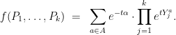
 ”, the function
  ,
, ![\displaystyle {\mathrm{Pr}}[~ \textstyle \sum_i X_i \geq \alpha ~] ~\leq~ {\mathrm E}\Big[ e^{-t \alpha} \prod_{j=1}^n e^{t X_j} \Big]. \ \ \ \ \ (1)](https://s0.wp.com/latex.php?latex=%5Cdisplaystyle+%7B%5Cmathrm%7BPr%7D%7D%5B%7E+%5Ctextstyle+%5Csum_i+X_i+%5Cgeq+%5Calpha+%7E%5D+%7E%5Cleq%7E+%7B%5Cmathrm+E%7D%5CBig%5B+e%5E%7B-t+%5Calpha%7D+%5Cprod_%7Bj%3D1%7D%5En+e%5E%7Bt+X_j%7D+%5CBig%5D.+%5C+%5C+%5C+%5C+%5C+%281%29&bg=ffffff&fg=000000&s=0&c=20201002)

![\displaystyle \begin{array}{rcl} {\mathrm E}_{X_{i+1},\ldots,X_n}[\: f(x_1,\ldots,x_i,X_{i+1},\ldots,X_n) \:] &=& e^{-t \alpha} \cdot \prod_{j=1}^i e^{t x_j} ~\cdot~ {\mathrm E}_{X_{i+1},\ldots,X_n}\Bigg[\: \prod_{j=i+1}^n e^{t X_j} \:\Bigg] \\ &=& e^{-t \alpha} \cdot \prod_{j=1}^i e^{t x_j} ~\cdot~ \prod_{j=i+1}^n {\mathrm E}_{X_j}\big[\: e^{t X_j} \:\big]. \end{array}](https://s0.wp.com/latex.php?latex=%5Cdisplaystyle+%5Cbegin%7Barray%7D%7Brcl%7D+%7B%5Cmathrm+E%7D_%7BX_%7Bi%2B1%7D%2C%5Cldots%2CX_n%7D%5B%5C%3A+f%28x_1%2C%5Cldots%2Cx_i%2CX_%7Bi%2B1%7D%2C%5Cldots%2CX_n%29+%5C%3A%5D+%26%3D%26+e%5E%7B-t+%5Calpha%7D+%5Ccdot+%5Cprod_%7Bj%3D1%7D%5Ei+e%5E%7Bt+x_j%7D+%7E%5Ccdot%7E+%7B%5Cmathrm+E%7D_%7BX_%7Bi%2B1%7D%2C%5Cldots%2CX_n%7D%5CBigg%5B%5C%3A+%5Cprod_%7Bj%3Di%2B1%7D%5En+e%5E%7Bt+X_j%7D+%5C%3A%5CBigg%5D+%5C%5C+%26%3D%26+e%5E%7B-t+%5Calpha%7D+%5Ccdot+%5Cprod_%7Bj%3D1%7D%5Ei+e%5E%7Bt+x_j%7D+%7E%5Ccdot%7E+%5Cprod_%7Bj%3Di%2B1%7D%5En+%7B%5Cmathrm+E%7D_%7BX_j%7D%5Cbig%5B%5C%3A+e%5E%7Bt+X_j%7D+%5C%3A%5Cbig%5D.+%5Cend%7Barray%7D+&bg=ffffff&fg=000000&s=0&c=20201002)
 (i.e., we know that
 ![{{\mathrm{Pr}}[ X_j=1 ] = p_j}](https://s0.wp.com/latex.php?latex=%7B%7B%5Cmathrm%7BPr%7D%7D%5B+X_j%3D1+%5D+%3D+p_j%7D&bg=ffffff&fg=000000&s=0&c=20201002) ).
). with
with  . Set
. Set ![{\mu = \sum_i {\mathrm E}[X_i]}](https://s0.wp.com/latex.php?latex=%7B%5Cmu+%3D+%5Csum_i+%7B%5Cmathrm+E%7D%5BX_i%5D%7D&bg=ffffff&fg=000000&s=0&c=20201002) ,
,  and
and  . We have
![\displaystyle {\mathrm{Pr}}[ \textstyle \sum_i X_i > (1+\delta) \mu ] ~\leq~ {\mathrm E}[ f(X_1,\ldots,X_n) ] ~\leq~ \exp\Big( - \mu \big( (1+\delta) \ln(1+\delta) - \delta\big) \Big),](https://s0.wp.com/latex.php?latex=%5Cdisplaystyle+%7B%5Cmathrm%7BPr%7D%7D%5B+%5Ctextstyle+%5Csum_i+X_i+%3E+%281%2B%5Cdelta%29+%5Cmu+%5D+%7E%5Cleq%7E+%7B%5Cmathrm+E%7D%5B+f%28X_1%2C%5Cldots%2CX_n%29+%5D+%7E%5Cleq%7E+%5Cexp%5CBig%28+-+%5Cmu+%5Cbig%28+%281%2B%5Cdelta%29+%5Cln%281%2B%5Cdelta%29+-+%5Cdelta%5Cbig%29+%5CBig%29%2C+&bg=ffffff&fg=000000&s=0&c=20201002)
 and
and  . We now apply the same argument as in
 ![\displaystyle \begin{array}{rcl} {\mathrm{Pr}}[~ \textstyle \sum_i X_i \geq (1+\delta) \mu ~|~ X_1=x_1,\ldots,X_n=x_n ~] &\leq& {\mathrm E}\Big[ f(X_1,\ldots,X_n) ~|~ X_1=x_1,\ldots,X_n=x_n \Big] \\ &=& f(x_1,\ldots,x_n) ~<~ 1. \end{array}](https://s0.wp.com/latex.php?latex=%5Cdisplaystyle+%5Cbegin%7Barray%7D%7Brcl%7D+%7B%5Cmathrm%7BPr%7D%7D%5B%7E+%5Ctextstyle+%5Csum_i+X_i+%5Cgeq+%281%2B%5Cdelta%29+%5Cmu+%7E%7C%7E+X_1%3Dx_1%2C%5Cldots%2CX_n%3Dx_n+%7E%5D+%26%5Cleq%26+%7B%5Cmathrm+E%7D%5CBig%5B+f%28X_1%2C%5Cldots%2CX_n%29+%7E%7C%7E+X_1%3Dx_1%2C%5Cldots%2CX_n%3Dx_n+%5CBig%5D+%5C%5C+%26%3D%26+f%28x_1%2C%5Cldots%2Cx_n%29+%7E%3C%7E+1.+%5Cend%7Barray%7D+&bg=ffffff&fg=000000&s=0&c=20201002)
 ”, there is no randomness remaining. The sum
  is not a random variable; it is simply the number
  . Since the event “
 ” has probability less than
 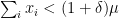 .
. . But the method is useful because we can apply it in more complicated scenarios that involve multiple Chernoff bounds.
 approximation to the congestion minimization problem. We now get a deterministic algorithm by the method of pessimistic estimators.
 with
with  of pairs of vertices. We want to find
  –
– paths such that each arc
  is contained in few paths. Let
  , we create a variable
  .
.
 with probability
  . For every arc
  be the indicator of the event “
 ”. Then the congestion on arc
  . We showed that
 ![{{\mathrm E}[ Y^a ] \leq C^*}](https://s0.wp.com/latex.php?latex=%7B%7B%5Cmathrm+E%7D%5B+Y%5Ea+%5D+%5Cleq+C%5E%2A%7D&bg=ffffff&fg=000000&s=0&c=20201002) . Let
. Let  . We applied Chernoff bounds to every arc and a union bound to show that
![\displaystyle {\mathrm{Pr}}[~ \mathrm{any} ~a~ \mathrm{has}~ Y^a > \alpha C^* ~] ~\leq~ \sum_{a \in A} {\mathrm{Pr}}[~ Y^a > \alpha C^* ~] ~\leq~ 1/n.](https://s0.wp.com/latex.php?latex=%5Cdisplaystyle+%7B%5Cmathrm%7BPr%7D%7D%5B%7E+%5Cmathrm%7Bany%7D+%7Ea%7E+%5Cmathrm%7Bhas%7D%7E+Y%5Ea+%3E+%5Calpha+C%5E%2A+%7E%5D+%7E%5Cleq%7E+%5Csum_%7Ba+%5Cin+A%7D+%7B%5Cmathrm%7BPr%7D%7D%5B%7E+Y%5Ea+%3E+%5Calpha+C%5E%2A+%7E%5D+%7E%5Cleq%7E+1%2Fn.+&bg=ffffff&fg=000000&s=0&c=20201002)
![\displaystyle \textstyle {\mathrm{Pr}}[~ \mathrm{any} ~a~ \mathrm{has}~ Y^a > \alpha C^* ~] ~\leq~ \sum_{a \in A} {\mathrm{Pr}}[~ Y^a > \alpha C^* ~] ~\leq~ {\mathrm E}[ f(P_1,\ldots,P_k) ] ~\leq~ 1/n.](https://s0.wp.com/latex.php?latex=%5Cdisplaystyle+%5Ctextstyle+%7B%5Cmathrm%7BPr%7D%7D%5B%7E+%5Cmathrm%7Bany%7D+%7Ea%7E+%5Cmathrm%7Bhas%7D%7E+Y%5Ea+%3E+%5Calpha+C%5E%2A+%7E%5D+%7E%5Cleq%7E+%5Csum_%7Ba+%5Cin+A%7D+%7B%5Cmathrm%7BPr%7D%7D%5B%7E+Y%5Ea+%3E+%5Calpha+C%5E%2A+%7E%5D+%7E%5Cleq%7E+%7B%5Cmathrm+E%7D%5B+f%28P_1%2C%5Cldots%2CP_k%29+%5D+%7E%5Cleq%7E+1%2Fn.+&bg=ffffff&fg=000000&s=0&c=20201002)
 for which
  . Thus,
![\displaystyle \begin{array}{rcl} {\mathrm{Pr}}[~ \mathrm{any} ~a~ \mathrm{has}~ Y^a > \alpha C^* \:|\: P_1=p_1,\ldots,P_k=p_k ~] &\leq& {\mathrm E}[~ f(P_1,\ldots,P_k) \:|\: P_1=p_1,\ldots,P_k=p_k ~] \\ &=& f(p_1,\ldots,p_k) ~\leq~ 1/n. \end{array}](https://s0.wp.com/latex.php?latex=%5Cdisplaystyle+%5Cbegin%7Barray%7D%7Brcl%7D+%7B%5Cmathrm%7BPr%7D%7D%5B%7E+%5Cmathrm%7Bany%7D+%7Ea%7E+%5Cmathrm%7Bhas%7D%7E+Y%5Ea+%3E+%5Calpha+C%5E%2A+%5C%3A%7C%5C%3A+P_1%3Dp_1%2C%5Cldots%2CP_k%3Dp_k+%7E%5D+%26%5Cleq%26+%7B%5Cmathrm+E%7D%5B%7E+f%28P_1%2C%5Cldots%2CP_k%29+%5C%3A%7C%5C%3A+P_1%3Dp_1%2C%5Cldots%2CP_k%3Dp_k+%7E%5D+%5C%5C+%26%3D%26+f%28p_1%2C%5Cldots%2Cp_k%29+%7E%5Cleq%7E+1%2Fn.+%5Cend%7Barray%7D+&bg=ffffff&fg=000000&s=0&c=20201002)
 ” must have probability
  then every arc
  , as desired.